Convex Optimization by convexjlr

The aim of package convexjlr is to provide optimization results rapidly and reliably in R once you formulate your problem as a convex problem. Having this in mind, we write this vignette in a problem-oriented style. The vignette will walk you through several examples using package convexjlr:

Lasso;
Logistic regression;
Support Vector Machine (SVM);
Smallest circle covering multiple points.

Although these problems already have mature solutions, the purpose here is to show the wide application of convex optimization and how you can use convexjlr to deal with them easily.

Some of the examples here are of statistics nature (like Lasso and logistic regression), and some of the examples here are of machine-learning nature (like SVM), they may be appealing to readers with certain backgrounds. If you don’t know either of this, don’t be afraid, the smallest circle problem requires no certain background knowledge.

We hope you can get ideas for how to use convexjlr to solve your own problems by reading these examples. If you would like to share your experience on using convexjlr, don’t hesitate to contact me: cxl508@psu.edu.

Knowledge for convex optimization is not necessary for using convexjlr, but it will help you a lot in formulating convex optimization problems and in using convexjlr.

Wikipedia page for convex optimization is a good starting point.
Github page for Convex.jl can give you more information for Convex.jl, which convexjlr is built upon.

To use package convexjlr, we first need to attach it and do some initial setup:

## sed seed for reproduciblity
set.seed(123)

library(convexjlr)

## 
## Attaching package: 'convexjlr'

## The following object is masked from 'package:base':
## 
##     norm

convex_setup(backend = "JuliaCall")

## Doing initialization. It may take some time. Please wait.

## Julia version 1.0.2 at location /Applications/Julia-1.0.app/Contents/Resources/julia/bin will be used.

## Loading setup script for JuliaCall...

## Finish loading setup script for JuliaCall.

## [1] TRUE

Lasso

Lasso is a variable selection and coefficient estimation method for linear regression. Interested reader can see the Lasso Page and the Wikipedia page Lasso (statistics) for more information.

Let us first see the lasso function using convexjlr:

lasso <- function(x, y, lambda){
    p <- ncol(x)
    ## n is a scalar, you don't have to use J(.) to send it to Julia.
    n <- nrow(x) ## n <- J(nrow(x))
    ## lambda is a scalar, you don't have to use J(.) to send it to Julia.
    ## lambda <- J(lambda)
    ## x is a matrix and y is a vector, you have to use J(.) to send them to Julia.
    x <- J(x)
    y <- J(y)
    ## coefficient vector beta and intercept b.
    beta <- Variable(p)
    b <- Variable()
    ## MSE is mean square error.
    MSE <- Expr(sumsquares(y - x %*% beta - b) / n)
    ## the L-1 penalty term of Lasso.
    penalty <- Expr(lambda * sum(abs(beta)))
    ## In Lasso, we want to minimize the sum of MSE and penalty.
    p1 <- minimize(MSE + penalty)
    cvx_optim(p1)
    list(coef = value(beta), intercept = value(b))
}

In the function, x is the predictor matrix, y is the response we have, lambda is the positive tuning parameter which controls the sparsity of the estimation. And the lasso function will return the coefficient and intercept solved by cvx_optim.

Now we can see a little example using the lasso function we have just built.

n <- 1000
p <- 100
## Sigma, the covariance matrix of x, is of AR-1 structure.
Sigma <- outer(1:p, 1:p, function(i, j) 0.5 ^ abs(i - j))
x <- matrix(rnorm(n * p), n, p) %*% chol(Sigma)
## The real coefficient is all zero except the first, second and fourth elements.
beta0 <- rep(0, p)
beta0[1:4] <- c(5, 1, 0, 2)
y <- x %*% beta0 + 0.2 * rnorm(n)

betahat <- round(lasso(x, y, 0.5)$coef, 4)
betahat[1:4]

## [1] 4.8192 0.9062 0.0000 1.8094

## You can see that the rest elements of betahat are all zero.
all(betahat[5:p] == 0)

## [1] TRUE

Logistic Regression

Logistic regression is a widely used method in Generalized Linear Model (GLM) to deal with binary response. Interested reader can see the Wikipedia page Logistic regression for more information.

Let us first see the logistic_regression function using convexjlr:

logistic_regression <- function(x, y){
    p <- ncol(x)
    ## x is a matrix and y is a vector, you have to use J(.) to send them to Julia.
    x <- J(x)
    y <- J(y)
    ## beta is the coefficient.
    beta <- Variable(p)
    ## sum(y * (x %*% beta)) - sum(logisticloss(x %*% beta))
    ## is the log-likelihood for logistic regressio,
    ## logisticloss(x) = log(1+exp(x)).
    p1 <- maximize(sum(y * (x %*% beta)) - sum(logisticloss(x %*% beta)))
    cvx_optim(p1)
    value(beta)
}

In the function, x is the predictor matrix, y is the binary response we have (we assume it to be 0-1 valued).

We first construct the log-likelihood of the logistic regression, and then we use cvx_optim to maximize it. Note that in formulating the log-likelihood, there is a little trick: we use logisticloss(x %*% beta) instead of log(1+exp(x %*% beta)), that is because logisticloss(.) is a convex function but by rule of Disciplined Convex Programming (DCP), we are not sure whether log(1+exp(.)) is convex or not. Interested readers can use ?operations or check http://convexjl.readthedocs.io/en/stable/operations.html for a full list of supported operations.

Now we can see a little example using the logistic_regression function we have just built.

n <- 500
p <- 2
## Sigma, the covariance matrix of x, is of AR-1 strcture.
Sigma <- outer(1:p, 1:p, function(i, j) 0.5 ^ abs(i - j))
x <- matrix(rnorm(n * p), n, p) %*% chol(Sigma)
## the real logistic regression coefficient.
beta0 <- c(1, -1)
## the probability for y = 1.
p0 <- 1 / (1 + exp(-x %*% beta0 + 0.2 * rnorm(n)))
y <- runif(n) < p0

logistic_regression(x, y)

##            [,1]
## [1,]  0.9723167
## [2,] -0.9953277

Support Vector Machine

Support vector machine (SVM) is a classification tool. In this vignette, we just focus on the soft-margin linear SVM. Interested reader can read more about SVM in the Wikipedia page Support vector machine.

Let us first see the svm function using convexjlr:

svm <- function(x, y, lambda){
    p <- ncol(x)
    ## n is a scalar, you don't have to use J(.) to send it to Julia.
    n <- nrow(x) ## n <- J(nrow(x))
    ## lambda is a scalar, you don't have to use J(.) to send it to Julia.
    ## lambda <- J(lambda)
    ## x is a matrix and y is a vector, you have to use J(.) to send them to Julia.
    x <- J(x)
    y <- J(y)
    ## w and b define the classification hyperplane <w.x> = b.
    w <- Variable(p)
    b <- Variable()
    ## hinge_loss, note that pos(.) is the positive part function.
    hinge_loss <- Expr(sum(pos(1 - y * (x %*% w - b))) / n)
    p1 <- minimize(hinge_loss + lambda * sumsquares(w))
    cvx_optim(p1)
    list(w = value(w), b = value(b))
}

In the function, x is the predictor matrix, y is the binary response we have (we assume it to be of negative one or one in this section). lambda is the positive tuning parameter which determines the tradeoff between the margin-size and classification error rate. As lambda becomes smaller, the classification error rate is more important. And the svm function will return the w and b which define the classification hyperplane as <w, x> = b.

Now we can see a little example using the svm function we have just built.

n <- 100
p <- 2
## Sigma, the covariance matrix of x, is of AR-1 structure.
Sigma <- outer(1:p, 1:p, function(i, j) 0.5 ^ abs(i - j))
## We generate two groups of points with same covariance and different mean.
x1 <- 0.2 * matrix(rnorm(n / 2 * p), n / 2, p) %*% chol(Sigma) + outer(rep(1, n / 2), rep(0, p))
x2 <- 0.2 * matrix(rnorm(n / 2 * p), n / 2, p) %*% chol(Sigma) + outer(rep(1, n / 2), rep(1, p))
x <- rbind(x1, x2)
## the label for the points.
y <- c(rep(1, n / 2), rep(-1, n / 2))

r <- svm(x, y, 0.5)
r

## $w
##            [,1]
## [1,] -0.4798997
## [2,] -0.4827123
## 
## $b
## [1] -0.4261342

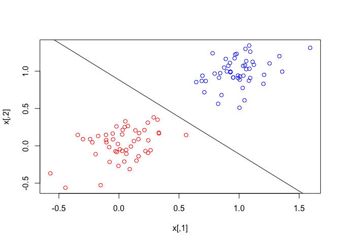
## We can scatter-plot the points and
## draw the classification hyperplane returned by the function svm.
plot(x, col = c(rep("red", n / 2), rep("blue", n / 2)))
abline(r$b / r$w[2], -r$w[1] / r$w[2])

Smallest Circle

In the last section of the vignette, let us see an example without any background knowledge requirement.

Suppose we have a set of points on the plane, how can we find the smallest circle that covers all of them? By using convexjlr, the solution is quite straight-forward.

if (!requireNamespace("plotrix", quietly = TRUE)) {
    stop("Package plotrix needed for this section of vignette to build. Please install it.")
}

center <- function(x, y){
    ## x and y are vectors of coordinates of the points,
    ## since they are vectors, we need to use J(.) to send them to Julia.
    x <- J(x)
    y <- J(y)
    ## Suppose the center of the smallest circle is p: (p[1], p[2]).
    p <- Variable(2)
    ## The square of radius of the circle that covers all the points
    ## is maximum((x - p[1]) ^ 2 + (y - p[2]) ^ 2).
    r2 <- Expr(maximum(square(x - p[1]) + square(y - p[2])))
    ## We want to minimize r2.
    p1 <- minimize(r2)
    cvx_optim(p1)
    value(p)
}

In the function, x and y are vectors of coordinates of the points. And the center function will return the coordinates of the center of the smallest circle that covers all the points.

Now we can see a little example using the center function we have just built.

n <- 20
## Generate some random points.
x <- rnorm(n)
y <- rnorm(n)

p <- center(x, y)
p

##            [,1]
## [1,] -0.4686643
## [2,]  0.2271158

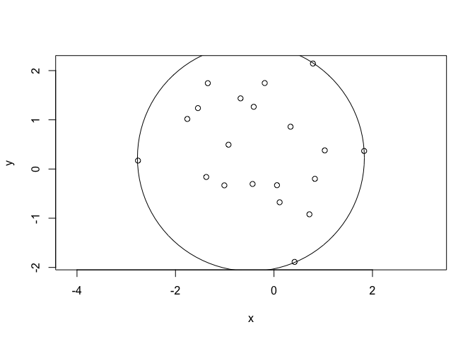
## Draw the points and the smallest circle that covers all of them.
plot(x, y, asp = 1)
plotrix::draw.circle(p[1], p[2], radius = sqrt(max((x - p[1]) ^ 2 + (y - p[2]) ^ 2)))

Changcheng Li

2018-12-16

Lasso

Logistic Regression

Support Vector Machine

Smallest Circle

Contents